Hello! If you are someone who deals with large volumes of video data who is interested in building a semantic layer on top for fuzzy querying with general understanding this article is for you.
Sieve works with billions of videos we procure through our own video collection platform, operations partners, and other data licensing partnerships. At Sieve, one of our main focuses is filtering down large corpora for concepts like “animals” or “instruments”. In the landscape of embedding search, it has traditionally been used for getting the most similar candidates, aka nearest-neighbours. We did not build a billion-video nearest-neighbor product rather we built a cheap, high-recall coarse filter that reduces the volume sent to a more expensive verifier.
My name is Sarina and this summer one of my biggest projects was embedding 1 billion videos in order to create novel ways to query categories of videos like “animals” or “instruments” and understand data distributions of video at scale and this is my account of the design, experiments and intuition behind it.
Embedding: turning data into vectors, similarity between vectors is measured based on varying types of distance measurements, e.g cosine distance.
Motivation, what’s the alternative?
Before diving into how to actually embed so many videos, the current approaches and most intuitive methods come to mind as follows (at least, this is where I start, then the approach evolved from there):
- Searching via metadata: While it is true that metadata (like titles, tags, etc) will get you 80% of the way there, sometimes there will be nuances in videos that aren’t caught. For example, “Acid-base Neutralization” is a well labelled video regarding science experiments, but searching for “science” will not surface this. Semantic intent is sometimes not captured in the title nor the captions and the visual space is very rich.
- Use off-the-shelf embedding API (as of July 2026): Gemini’s embedding model (
gemini-embedding-2) allows for multimodal projection into the same embedding space, but the economics become challenging at scale. Gemini’s documented video-input path samples uniformly up to 32 frames for longer videos, which would not preserve every moment in an average 15.2-minute video. To retain a denser temporal view, we would need to sample frames ourselves: for example, 1 fps gives roughly 912 images per average video. If we submit them through the input path, at the current Gemini Embedding 2 image-input price of $0.00012 per image, that comes out to 912 × 1,000,000,000 × $0.00012 ≈ $109.4 million before any volume discounts. That is still prohibitive at our scale.
So, there is clear precedent for building our own local embedding model runtime, fit with a model, filtering algorithms and optimized for performance.
Choosing a model and a runtime
There are a multitude of cloud GPUs and many, many embedding models out there. Breaking this down by model and runtime:
Model
For our specific needs, we opt for SigLIP2, due to prior work on this model and in our case, we wanted models that specialize in text → image retrieval. If not SigLIP2, it would have been another model with CLIP capabilities, (Contrastive Language-Image Pretraining; combining text and other modalities into the same subspace).
Some other models you can consider: MetaCLIP 2, EVA-CLIP
Runtime
We opt for L4 GPU with higher CPU specs for preprocessing because the throughput is acceptable enough given the compute cost, and we can scale horizontally. Thus a beefier, larger GPU (like H100, A100 etc) was not needed. Read about more options here, from Google’s offerings. We opt for preemptable nodes offering a 60-70% discount.
Methodology & measuring cost and performance
What to embed exactly?
The simplest way and most intuitive way to embed a video is to uniformly sample frames then embed those frames, treating them as images and attaching a timestamp on them. But there are costs at scale with network bandwidth, dealing with such large volumes of data, etc. There are alleviations such as downscaling videos, or preprocessing your corpus and shrinking it down to numerous thumbnails representing a video, then downloading those objects and using those as your uniformly sampled frames.
Information deduplication
Uniform sampling comes with it’s own set of problems:
- You miss scenes if your fps is too low
- You sample too many redundant frames
But the second is actually easier to fix than the first through some smart frame deduplication, so it’s better to sample at a higher fps, then prune. The key here is to identify “pivotal” moments, which we define as scene changes, unique environments or colour scheme changes.
To identify pivotal moments, you can start with a perceptual hashing algorithm like difference hashing and take hashes whose hamming distance is bigger than an arbitrary threshold from every other frame previously kept. In other words, process frames that are more different from each other than an arbitrary threshold.
In our case, we find that a hamming distance of 15 worked best for us in terms of filtering that was nuanced enough but pruned out visually similar duplicates. Perceptual hashing is very useful for detecting and pruning structurally similar frames, such as scene cuts and different faces or places. But what it lacks is nuance to long tail transitions, pans and gradual changes, which can end up keeping nearly every frame and not being much better.
As a result, we layer one more algorithm on top to deal with these gradual transitions, using a colour histogram. For every frame, we compute both a difference hash and a 96-dim RGB histogram (32 bins × 3). The difference hash is still the first gate: if a frame is not structurally different enough from the frames we have already kept, we skip it immediately. Only when the difference hash passes that threshold do we check the colour histogram against a sliding window of the last 10 frames overall, not just the frames selected by difference hash. We keep the frame only if its minimum χ²-distance from every histogram in that window is ≥ 0.05. After each frame, the window slides forward.
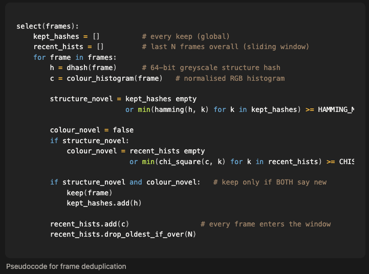
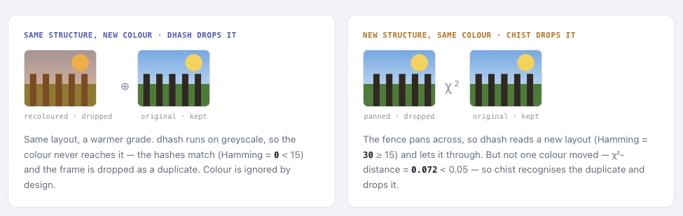
Both these layers are complementary to one another, difference hashing handling the genuine structural changes and colour histogram handling gradual transitions.
With our pruning method, we select only on average ~29.3% of all frames! Extreme cases select/keep 86% of frames or select/keep 0.7% of frames. Long videos skew the mean higher, the median video selects/keeps ~20.3% of its frames.
Evaluating this (see below on recall & precision evaluation methodology) retains nearly the exact same recall and precision to prune out nearly 67% of all frames, which shows that majority of uniform sampling is redundant, but information deduplication before anything touches a GPU can save a lot at scale.
Recall and precision
During our process of picking embedding strategies, one of the most important things was having a good evaluation harness, in this case was figuring out our precision and recall on all of our experiments to determine the quality of the method.
In our case, we do not use recall@k because we do not want k videos, we want whatever video fits a query, below a certain cosine distance threshold. The reason we change our criteria for correctness is to match our requirements of this system, which is to sift through a large volume of videos to fuzzy match a semantic query rather than picking the most accurate “top k” candidates. Additionally, building an index on billions of videos may require onboarding vector databases to build an index at this scale or clever engineering work to maintain such an index at a scale.
(see querying embeddings for more information)
Let’s define the oracle in this case is a video selected by some criteria; if I say I want videos of animals, a video with animals is an oracle video. A selected video will refer to a video that meets an arbitrary cosine distance threshold after encoding a query against our embeddings.
Start by defining our confusion matrix:
| Is an oracle video (all oracle) | Is not an oracle video (everything else) | |
|---|---|---|
| is selected (lower than the cosine distance threshold) | True positive | False positive |
| is not selected (higher or equal to the cosine distance threshold) | False negative | True negative |
and then the metrics we care about in our context:
Recall: TP / (TP+FN) → is oracle and is selected / all oracle videos
Precision: TP / (TP+FP) → is oracle and is selected / all selected videos
- Recall determines the expected yield of data as we scale the input corpus, and a general feel for the data distribution (like what percentage of videos qualify at progressively tighter and tighter thresholds) but picking a loose cosine distance threshold for would be enough to increase this metric
- Precision is helpful in benchmarking the general quality of the embedding method but we tradeoff with recall when loosening the cosine threshold since we select more videos
Recall becomes useful alongside pass rate because together they show the tradeoff between retained yield and downstream cost. Here is an example of how these metrics direct the work here:
Suppose our production pipeline costs $2 to run per video. Fine-grained (fg) is our only source of ground truth: it's the sole step that actually confirms whether a video is a true positive, so without any pre-filter, the only way to hit our yield target is to run every one of our 1,000,000 videos through fg: $2 × 1,000,000 = $2,000,000, just to find out which ones are true positives.
Now say I set the cosine distance threshold to 0.88. At that threshold, the coarse embedding filter has 60% recall and a 29% pass rate. In other words, it retains about 60% of the true positives that exist in the corpus, while only sending 29% of the total corpus downstream to the fine-grained pipeline.
- I run the same 1,000,000-video corpus through the coarse filter first, as a cheap pre-pass over what I already have.
- Only 290,000 videos clear the threshold and get sent to the $2/video fg pipeline, so my fg spend drops from $2,000,000 to $580,000.
- The remaining 710,000 videos avoid fine-grained processing, which is where the 71% cost reduction comes from.
The tradeoff is between retained qualifying yield and avoided fine-grained processing: by choosing this threshold, I keep around 60% of the true positives, but I avoid running the expensive pipeline on 71% of the corpus. Recall tells me how much qualifying yield survives; pass rate tells me how much downstream work remains.
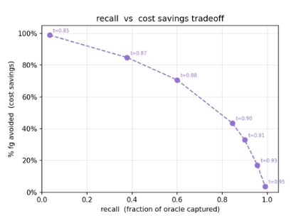
And then, with this evaluation in mind, you pick different embedding, information deduplication and querying methods to measure and benchmark its performance.
Fun fact: the entire colour histogram, difference hashing algorithm produced retains nearly the exact same cost recall curve, at recall 60%, we avoid 62% of the corpus instead of the 71% shown in the example above!
Storing and querying billions of embeddings
Our embeddings are 768 dim, fp32, this is what SigLIP2 natively outputs. Naively, you can start by storing this directly into a database table. This is fine, and you can make this more efficient by constructing an index (using pgvector for example, if on Postgres or Clickhouse’s vector search mechanics) to query for top k candidates. But in situations where the average number of embeddings for a video is 41.2, you'll end up with 41.2B vectors to query. Some quick napkin math on what that costs using HNSW at 768-dim fp32:
Memory: 41.2B × 768 × 4 bytes ≈ 126.6TB (with f32 quantization) for raw vectors, plus ~10.5TB of graph overhead → ~137.1TB total. That's far beyond what fits in RAM on any single machine, so the index ends up disk-bound or sharded across dozens of high-memory hosts before a single query even runs.
Index overhead: ClickHouse’s vector similarity index uses HNSW, and its hnsw_max_connections_per_layer parameter is the HNSW M value. The default is M=32, and ClickHouse estimates in-memory graph cost as num_vectors × M × 4 bytes × 2. For 41.2B vectors, that is roughly 10.5TB of graph memory before extra runtime buffers and caches. ClickHouse also notes that vector indexes must be fully loaded into memory for search, so this is not just a disk storage problem.
At this scale, maintaining an ANN index for top-k search would require a memory footprint and operational budget that did not make sense for our use case, especially because our goal is not nearest-neighbor retrieval but coarse threshold filtering.
You could also specialized vector database (like Pinecone or Qdrant) which construct a sharded index for you at scale to query at scale, but we opt for a slightly different approach because of different requirements:
Recall that we do not care about top k candidates, and our use case for embeddings is a general pre-filter, as a result, we actually do not need an index at all, rather we can afford to directly store the embedding as a regular column. But we need not to pull 41.2B vectors into memory at once, because cosine distance threshold is absolute for any query and does not care about its neighbours like top k does. As a result, we simply break down a large requirement of input into sample queries or using hashes to shard, then perform brute force cosine distance comparison. Using some more napkin math to show how we can get hundreds of millions in results with a db like Clickhouse, which excels at this type of query:
Row cost: 768 × 4 bytes = 3,072 bytes/row for siglip2_frame_embedding_768, plus a bit for the other selected columns, call it ~3.1KB/row
Throughput: cosineDistance is memory-bandwidth-bound, not compute-bound, the dot-product math (~3,000 FLOPs/row) is cheap next to just moving 3.1KB/row through memory. A well-provisioned single ClickHouse node with ~200GB/s aggregate memory bandwidth can push:
200e9 bytes/s ÷ 3,100 bytes/row ≈ ~65M rows/sec
Query time at that rate:
A "hundreds of millions" sample, say 500M rows, gives an idealized memory-bandwidth ceiling: 500e6 ÷ 65e6 ≈ 7.7 seconds, assuming the data is effectively memory-resident and the scan sustains ~200GB/s. Real query time will depend on storage, compression, cache behavior, and ClickHouse query overhead. The key architectural point is that these scans can be split across mutually exclusive shards because cosine-distance thresholding is independent per embedding; it does not require a global nearest-neighbor index.
Notes:
- You can quantize embeddings to bf16 or lower precision, but we don’t need to. This can halve memory requirements
- During query encoding time we found what works best for us is to have variations of a query in English, then take the minimum cosine distance for any query. This method was the most robust because it encoded variation that helped with very narrow queries (like “talking head” was complemented with “interviewer” or “person talking to a camera”)
- Encoding the text query can be directly done on CPU sidecar service alongside our internal services very cheaply
Takeaways
So, here are some mistakes and things that I wish I knew that I know now after doing all of this experimentation to determine feasibility:
- Input pruning is the strongest form of efficiency increase, having less to process made everything downstream less difficult when optimizing
- Chasing multiple modalities (like audio, captions) don’t work as well as focusing on making one very sturdy slice of semantic understanding, but will work as a complementary layer after one has been established. Likely should share separate query paths instead of collapsing them into the same subspace. It really boils down to the use case where real videos work best for visual, music for audio, text for podcast.
- Having an evaluation harness figured out at the start and staying consistent with the same oracle, same corpus and metrics will make everything downstream easier, but it’s not always easy to come up with good metrics the first time around until making some mistakes
- After figuring out feasibility in theory, in practicality things at scale don’t always work the way things are intended. (evident in my part 2, where I will cover how to write code that optimizes performance for heavy throughput embedding!)
Next steps
Some next steps for the embedding experimentation in the future:
- More effort and evaluation into different modalities and a dedicated harness for evaluating their effectiveness. For example, the visual method leaned heavily on looking for concepts like “nature”, “instruments”, “vehicles” or “talking heads”. Audio embeddings should get their equivalent harness / evaluation method
- Proper embedding versioning and handling of cases where we might want to migrate to another model of embeddings and how to reconcile both when querying and videos may only have one embedding or the other
- Experimentation with quantization and other methods of performance speed ups. We never had properly evaluated how quantizing the embeddings would impact performance, so this is an axis to leverage next time if things lean into cutting costs.
- Further in depth experimentation with query methodology (what defines a threshold, flexibility around the threshold, different methods to combine metadata and embeddings)
Stay tuned for part 2: building and writing code for a backfill task for billions of videos and frames, the mess behind performance optimization, discipline in observability, the importance of understanding OS fundamentals like processes, threads and contention, GPU maxxing!
PS: And if working on billion-scale multimodal indexing, fault-tolerant GPU backfills, and evaluation systems like these sounds interesting, we’re hiring across infrastructure, reliability, applied research, and machine learning.